Calculate the local time at the target location, as well as sunrise, sunset and solar noon times, and create several temporal masks.
The returned dataframe will have as many rows as the length of the incoming
UTC time vector and will contain the following columns:
localStdTime_UTC– UTC representation of local standard timedaylightSavings– logical mask = TRUE if daylight savings is in effectlocalTime– local clock timesunrise– time of sunrise on each localTime daysunset– time of sunset on each localTime daysolarnoon– time of solar noon on each localTime dayday– logical mask = TRUE between sunrise and sunsetmorning– logical mask = TRUE between sunrise and solarnoonafternoon– logical mask = TRUE between solarnoon and sunsetnight– logical mask = opposite of day
timeInfo(time = NULL, longitude = NULL, latitude = NULL, timezone = NULL)Arguments
Value
A dataframe with times and masks.
Details
NOAA used the reference below to develop their Sunrise/Sunset
https://gml.noaa.gov/grad/solcalc/sunrise.html and Solar Position
https://gml.noaa.gov/grad/solcalc/azel.html Calculators. The algorithms include corrections for atmospheric refraction effects.
Input can consist of one location and at least one POSIXct times, or one POSIXct time and at least one location. solarDep is recycled as needed.
Do not use the daylight savings time zone string for supplying dateTime, as many OS will not be able to properly set it to standard time when needed.
The localStdTime_UTC column in the returned dataframe is primarily for
internal use and provides an important tool for creating LST daily averages
and LST axis labeling.
Note
NOAA notes that “for latitudes greater than 72 degrees N and S, calculations are accurate to within 10 minutes. For latitudes less than +/- 72 degrees accuracy is approximately one minute.”
Attribution
Internal functions used for ephemerides calculations were copied verbatim from the now deprecated maptools package source code in an effort to reduce the number of package dependencies.
Warning
Compared to NOAA's original Javascript code, the sunrise and sunset estimates from this translation may differ by +/- 1 minute, based on tests using selected locations spanning the globe. This translation does not include calculation of prior or next sunrises/sunsets for locations above the Arctic Circle or below the Antarctic Circle.
Local Standard Time
US EPA regulations mandate that daily averages be calculated based on "Local Standard Time" (LST) (i.e. never shifting to daylight savings). To ease work in a regulatory context, LST times are included in the returned dataframe.
References
Meeus, J. (1991) Astronomical Algorithms. Willmann-Bell, Inc.
Examples
library(MazamaTimeSeries)

Carmel <-
  Carmel_Valley %>%
  mts_filterDate(20160801, 20160810)

# Create timeInfo object for this monitor
ti <- timeInfo(
  Carmel$data$datetime,
  Carmel$meta$longitude,
  Carmel$meta$latitude,
  Carmel$meta$timezone
)

t(ti[6:9,])
#>                       6                     7
#> localStandardTime_UTC "2016-08-01 04:00:00" "2016-08-01 05:00:00"
#> daylightSavings       "TRUE"                "TRUE"
#> localTime             "2016-08-01 05:00:00" "2016-08-01 06:00:00"
#> sunrise               "2016-08-01 06:13:45" "2016-08-01 06:13:45"
#> sunset                "2016-08-01 20:12:10" "2016-08-01 20:12:10"
#> solarnoon             "2016-08-01 13:13:13" "2016-08-01 13:13:13"
#> day                   "FALSE"               "FALSE"
#> morning               "FALSE"               "FALSE"
#> afternoon             "FALSE"               "FALSE"
#> night                 "TRUE"                "TRUE"
#>                       8                     9
#> localStandardTime_UTC "2016-08-01 06:00:00" "2016-08-01 07:00:00"
#> daylightSavings       "TRUE"                "TRUE"
#> localTime             "2016-08-01 07:00:00" "2016-08-01 08:00:00"
#> sunrise               "2016-08-01 06:13:45" "2016-08-01 06:13:45"
#> sunset                "2016-08-01 20:12:10" "2016-08-01 20:12:10"
#> solarnoon             "2016-08-01 13:13:13" "2016-08-01 13:13:13"
#> day                   "TRUE"                "TRUE"
#> morning               "TRUE"                "TRUE"
#> afternoon             "FALSE"               "FALSE"
#> night                 "FALSE"               "FALSE"

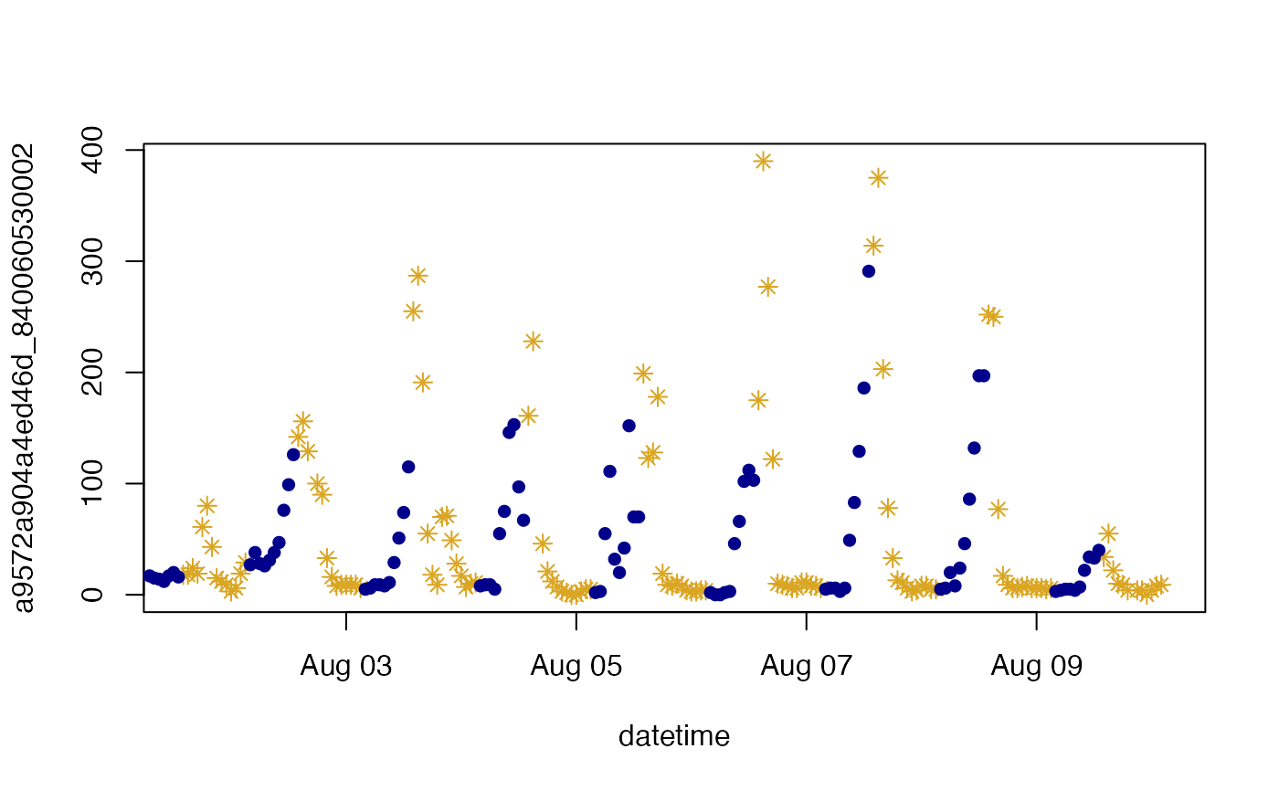
# Subset the data based on day/night masks
data_day <- Carmel$data[ti$day,]
data_night <- Carmel$data[ti$night,]

# Build two monitor objects
Carmel_day <- list(meta = Carmel$meta, data = data_day)
Carmel_night <- list(meta = Carmel$meta, data = data_night)

# Plot them
plot(Carmel_day$data, pch = 8, col = 'goldenrod')
points(Carmel_night$data, pch = 16, col = 'darkblue')
