Calculate the local time for the monitor, as well as sunrise, sunset and solar noon times, and create several temporal masks.
The returned dataframe will have as many rows as the length of the incoming
UTC time vector and will contain the following columns:
localStdTime_UTC-- UTC representation of local standard timedaylightSavings-- logical mask = TRUE if daylight savings is in effectlocalTime-- local clock timesunrise-- time of sunrise on each localTime daysunset-- time of sunset on each localTime daysolarnoon-- time of solar noon on each localTime dayday-- logical mask = TRUE between sunrise and sunsetmorning-- logical mask = TRUE between sunrise and solarnoonafternoon-- logical mask = TRUE between solarnoon and sunsetnight-- logical mask = opposite of day
monitor_timeInfo(ws_monitor = NULL, monitorID = NULL)
Arguments
| ws_monitor | ws_monitor object. |
|---|---|
| monitorID | Monitor ID for a specific monitor in |
Value
A dataframe with times and masks.
Details
While the lubridate package makes it easy to work in local timezones, there is no easy way in R to work in "Local Standard Time" (LST) as is often required when working with air qualitiy data. EPA regulations mandate that daily averages be calculated based on LST.
The localStdTime_UTC is primarily for use internally and provides
an important tool for creating LST daily averages and LST axis labeling.
Examples
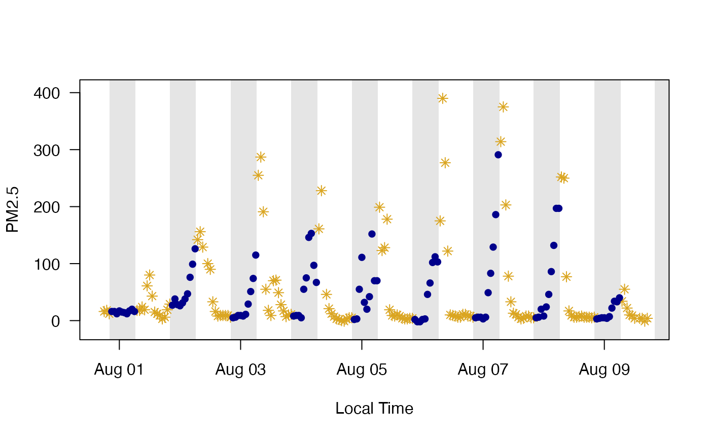
library(PWFSLSmoke) carmel <- monitor_subset(Carmel_Valley, tlim = c(20160801,20160810)) # Create timeInfo object for this monitor ti <- monitor_timeInfo(carmel) # Subset the data based on day/night masks data_day <- carmel$data[ti$day,] data_night <- carmel$data[ti$night,] # Build two monitor objects carmel_day <- list(meta = carmel$meta, data = data_day) carmel_night <- list(meta = carmel$meta, data = data_night) # Plot them monitor_timeseriesPlot(carmel_day, shadedNight = TRUE, pch = 8, col = 'goldenrod')
