Working With openair
Eli Grosman, Mazama Science
August 18, 2020
Source:vignettes/articles/Working_with_openair.Rmd
Working_with_openair.RmdBackground
The RAWSmet package was developed to make downloading and working with weather data gathered by RAWS stations simpler. Using this package in conjunction with the openair package can make some beautiful and informative visualizations of RAWS data.
openair is an R package designed specifically for modeling air quality data. The package provides many different tools for plotting wind and pollution roses, flexible time series plots, and more. Additionally, openair can easily group data and plot it by different periods such as by the hour, day, day of the week, season, and year. More information and documentation for openair may be found on its website: https://davidcarslaw.github.io/openair/.
The goal of this document is to introduce the use of RAWSmet and openair to create visualizations of weather data..
Setting up RAWSmet
Follow these instructions to set up RAWSmet correctly. These instruction may also be found on the package’s website: https://mazamascience.github.io/RAWSmet/.
To follow along with the rest of this document you may also install openair by running the following in the RStudio console:
install.packages("openair")The RAWSmet package is designed to be used with R (>= 3.5) and RStudio so make sure you have those installed first.
Users will want to install the remotes package to have access to the latest version of the package from GitHub.
The following packages should be installed by typing the following at the RStudio console:
# Note that vignettes require knitr and rmarkdown
install.packages('knitr')
install.packages('rmarkdown')
install.packages('MazamaSpatialUtils')
remotes::install_github('MazamaScience/MazamaLocationUtils')
remotes::install_github('MazamaScience/RAWSmet')
Any work with spatial data, e.g. assigning states, counties and timezones, will require installation of required spatial datasets. To get these datasets you should type the following at the RStudio console:
library(MazamaSpatialUtils)
dir.create('~/Data/Spatial', recursive = TRUE)
setSpatialDataDir('~/Data/Spatial')
installSpatialData()
Data generated with package functions can be be saved to and reloaded
from a dedicated directory much the same as the
spatialDataDir used above. Set up a directory for RAWS data
with:
library(RAWSmet)
dir.create('~/Data/RAWS', recursive = TRUE)
setRawsDataDir('~/Data/RAWS')
The rawsDataDir must be set up correctly to use its
functionality. RAWS data takes a long time to download so data may be
saved to this directory so it does not need to be downloaded again in
the future.
Preparing data for openair
Throughout this section, we will be using RAWSmet’s
cefa_load() and cefa_loadMeta() functions.
These functions will either load the specified data from
rawsDataDir or download and save it to the
rawsDataDir if it does not exist. You may also use
wrcc_loadYear() and wrcc_loadMeta() for RAWS
data from the WRCC.
Before using RAWS data with openair, we must ensure that the data is downloaded correctly and is in the correct format.
First, create or load all of the FW13 station metadata using
cefa_loadMeta().
library(RAWSmet)
library(MazamaSpatialUtils)

setSpatialDataDir("~/Data/Spatial")
setRawsDataDir("~/Data/RAWS")

meta <- cefa_loadMeta()
head(meta)
## # A tibble: 6 × 14
## deviceDeploymentID deviceID locationID locationName longitude latitude
## <chr> <chr> <chr> <chr> <dbl> <dbl>
## 1 f607cead84c92505_021503 021503 f607cead84c9… AHAKAHV PRE… -114. 34.1
## 2 68bd6497ac6c9cd9_500726 500726 68bd6497ac6c… ALCAN HWY M… -141. 62.8
## 3 31ccbb7f70c89629_020401 020401 31ccbb7f70c8… ALPINE -109. 33.8
## 4 df3cb89ae9f12826_500742 500742 df3cb89ae9f1… ANGEL CREEK… -146. 65.0
## 5 ff6ba96bd245b737_032101 032101 ff6ba96bd245… ARMSTEAD MT. -92.8 35.6
## 6 e67e4e384e4e5831_010702 010702 e67e4e384e4e… BANKHD -87.3 34.3
## # ℹ 8 more variables: elevation <dbl>, countryCode <chr>, stateCode <chr>,
## # timezone <chr>, nwsID <chr>, wrccID <chr>, nessID <chr>, agencyName <chr>The meta_leaflet() function provides an interactive map
to help find the ID associated with a particular location. Just click on
a dot to find the associated ID:
meta_leaflet(meta)We will choose the station in Enumclaw, Washington (451702) and create or load a “timeseries object”. This timeseries object contains two dataframes, one of station metadata and another of cleaned weather data.
# nwsID 451702 is Enumclaw, WA
Enumclaw <- cefa_load(nwsID = 451702, meta = meta)
## Loading data from /Users/jonathancallahan/Data/RAWS/cefa_451702_2023.rda
names(Enumclaw)## [1] "meta" "data"
# View station metadata
Enumclaw$meta
## # A tibble: 1 × 14
## deviceDeploymentID deviceID locationID locationName longitude latitude
## <chr> <chr> <chr> <chr> <dbl> <dbl>
## 1 277eac5c8aa229d6_451702 451702 277eac5c8aa2… ENUMCLAW -122. 47.2
## # ℹ 8 more variables: elevation <dbl>, countryCode <chr>, stateCode <chr>,
## # timezone <chr>, nwsID <chr>, wrccID <chr>, nessID <chr>, agencyName <chr>
# View sample of raw data
head(Enumclaw$data)
## # A tibble: 6 × 12
## datetime temperature humidity windSpeed windDirection maxGustSpeed
## <dttm> <dbl> <dbl> <dbl> <dbl> <dbl>
## 1 2004-01-06 19:00:00 8.3 28.5 4.9 170 8.9
## 2 2004-01-06 20:00:00 11.1 28.5 5.4 167 10.3
## 3 2004-01-06 21:00:00 13.9 28.5 4.5 165 12.1
## 4 2004-01-06 23:00:00 9.4 29 3.1 29 4
## 5 2004-01-07 00:00:00 8.3 34.5 3.1 25 4.9
## 6 2004-01-07 01:00:00 6.7 34.5 3.1 22 4.9
## # ℹ 6 more variables: maxGustDirection <dbl>, precipitation <dbl>,
## # solarRadiation <dbl>, fuelMoisture <dbl>, fuelTemperature <dbl>,
## # monitorType <chr>Note that this RAWS timeseries object contains all of the
data gathered by the specified station in its lifetime. We can filter
the data to look at periods of interest using
raws_filterDate(). This function can understand any date
that is understood by lubridate::ymd().
Also note that the data stored in these RAWS timeseries objects are in UTC.
# 20050101 will be parsed as Jan. 1st, 2005
# 20060101 will be parsed as Jan 1st. 2006

# Get all observations between these dates
Enumclaw_2005 <-
  raws_filterDate(Enumclaw,
                  startdate = 20050101,
                  enddate = 20060101,
                  timezone = "America/Los_Angeles")

range(Enumclaw_2005$data$datetime)
## [1] "2005-01-01 08:00:00 UTC" "2006-01-01 07:00:00 UTC"
# 20050801 will be parsed as Aug. 1st, 2005
# 20050901 will be parsed as Sep. 1st, 2005

# Get all observations between these dates
Enumclaw_200508 <-
  raws_filterDate(Enumclaw,
                  startdate = 20050801,
                  enddate = 20060901,
                  timezone = "America/Los_Angeles")

range(Enumclaw_200508$data$datetime)
## [1] "2005-08-01 07:00:00 UTC" "2006-09-01 06:00:00 UTC"Openair requires that dates and times of
observations are stored in a column called date. However,
RAWSmet names this column datetime. Use
raws_getData() with forOpenair = TRUE to
extract the data dataframe from a RAWS timeseries object
with a new column called date containing the same values as
datetime.
enumclawData_2005 <-raws_getData(Enumclaw_2005, forOpenair = TRUE)
enumclawData_200508 <-raws_getData(Enumclaw_2005, forOpenair = TRUE)
All of the functions used above may be used separately as
demonstrated but they can also be strung neatly together by using the
pipe %>% operator. The same data may be generated like
so:
meta <- cefa_loadMeta()

enumclawData_2005 <-
  cefa_load(nwsID = 451702, meta = meta) %>%
  raws_filterDate(20050101, 20060101, timezone = "America/Los_Angeles") %>%
  raws_getData(forOpenair = TRUE)

enumclawData_200508 <-
  cefa_load(nwsID = 451702, meta = meta) %>%
  raws_filterDate(20050801, 20050901, timezone = "America/Los_Angeles") %>%
  raws_getData(forOpenair = TRUE)

# We will also extract a dataframe of ALL of the station's data
enumclawData_ALL <-
  cefa_load(nwsID = 451702, meta = meta) %>%
  raws_getData(forOpenair = TRUE)
After renaming the datetime column and filtering by dates of interest, we are now ready to create visualizations using openair.
Using openair
The RAWS timeseries data contains measurements for temperature, humidity, wind speed, wind direction, max gust speed, max gust direction, precipitation, and solar radiation. We can utilize various openair plots to gain insight from each of these parameters.
Wind rose plots
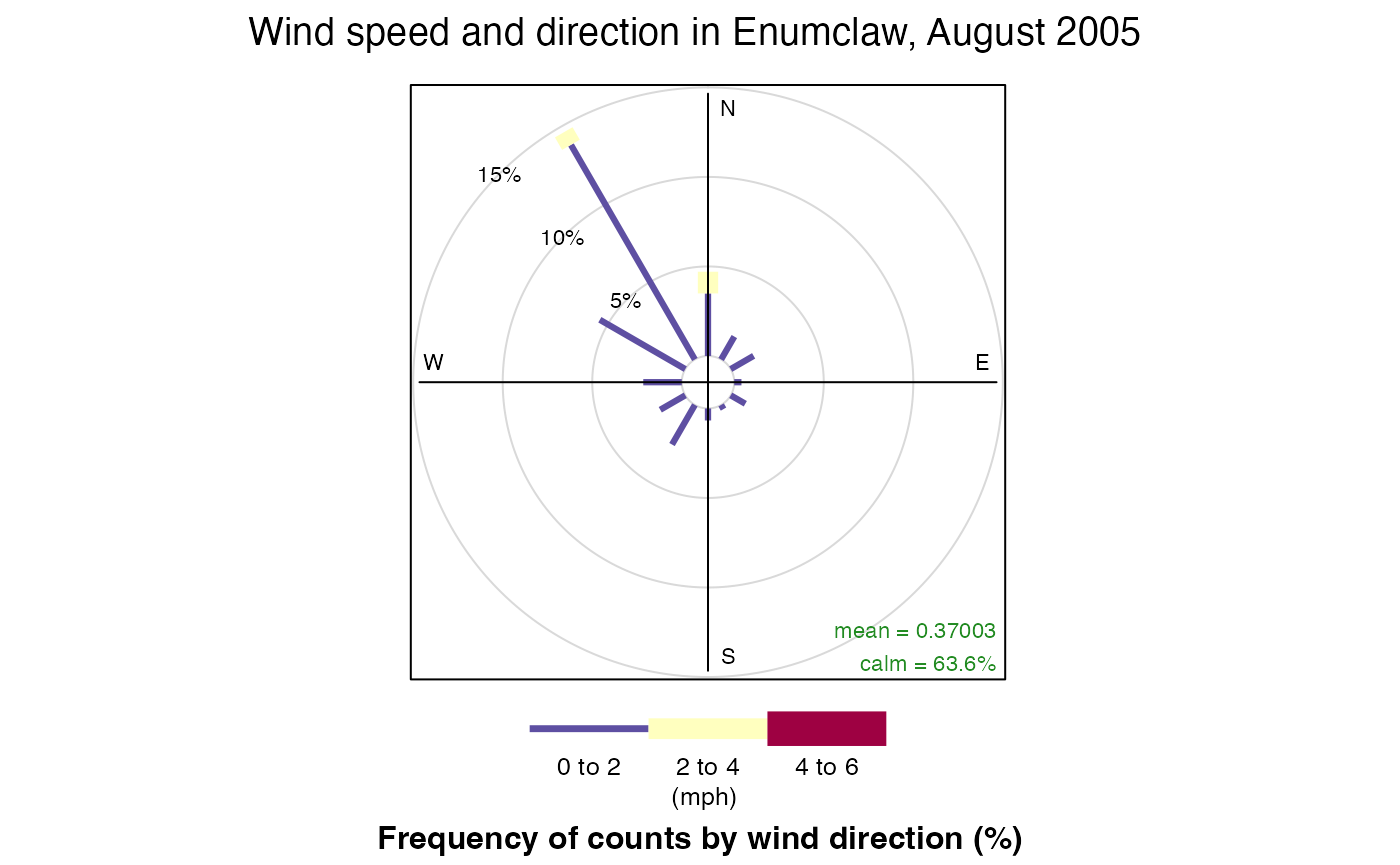
Let us first create some wind rose plots. Openair’s
windRose() function requires 3 arguments: the data to
create the plot for, and the names of the wind speed and wind direction
columns. By default, windRose() looks for columns named
ws and wd for wind speed and direction
respectively so it is important to specify these names when calling the
function. (Remember that openair requires that
dates and times of observations be stored in a column named
date.)
library(openair)

openair::windRose(
  enumclawData_200508,
  ws = "windSpeed",
  wd = "windDirection",
  main = "Wind speed and direction in Enumclaw, August 2005",
  key.footer = "(mph)"
)
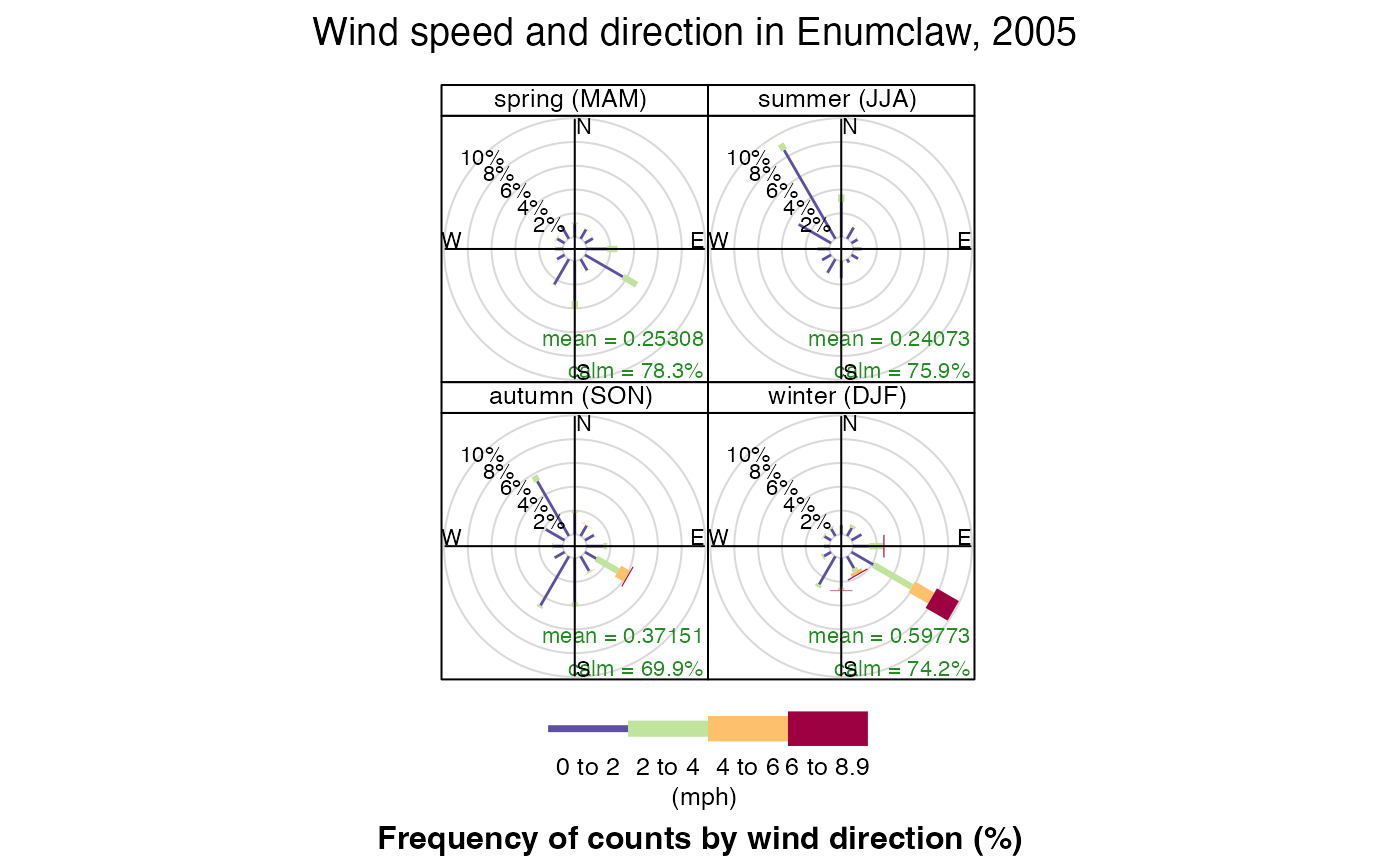
windRose() can also group data and plot it by different
periods. Lets look at the wind speed and directions by season in
Enumclaw:
openair::windRose(
  enumclawData_2005,
  ws = "windSpeed",
  wd = "windDirection",
  main = "Wind speed and direction in Enumclaw, 2005",
  type = "season",
  key.footer = "(mph)"
)
Time-series plotting
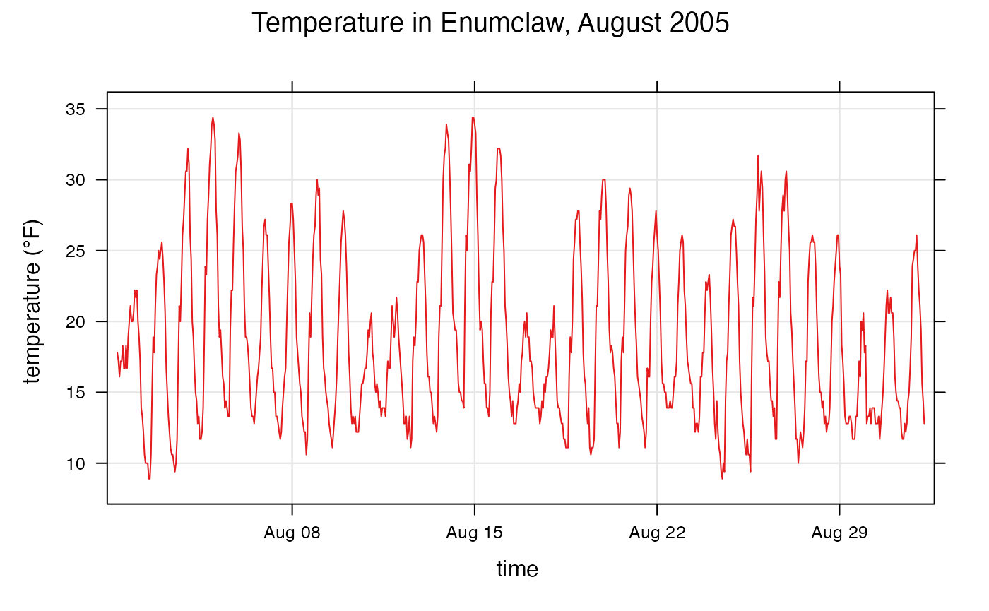
Openair can also be used to create time-series plots
and trends. Lets first take a look at the function
timePlot(). This function requires 2 arguments: the data to
create the plot for, and pollutant, the name of the column
to plot with respect to time. (Again, timePlot()
requires that dates and times of observations are stored in a column
named date.)
openair::timePlot(
  enumclawData_200508,
  pollutant = "temperature",
  avg.time = "hour",
  main = "Temperature in Enumclaw, August 2005",
  key = FALSE,
  xlab = "time",
  ylab = "temperature (°F)"
)
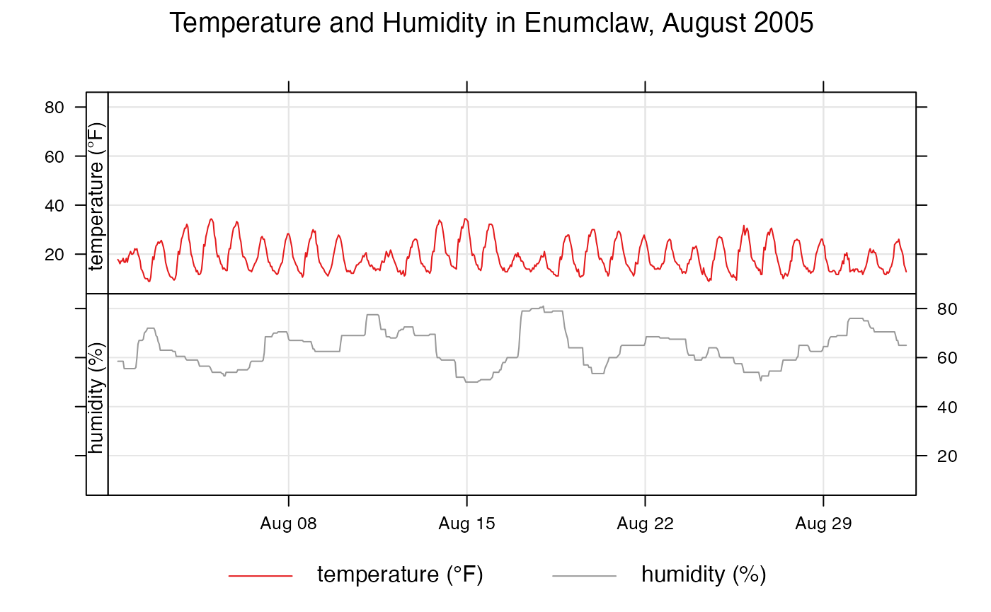
timePlot() can also plot multiple columns so they can be
compared against each other. Lets compare temperature and humidity in
Enumclaw in August 2005:
openair::timePlot(
  enumclawData_200508,
  pollutant = c("temperature", "humidity"),
  avg.time = "hour",
  main = "Temperature and Humidity in Enumclaw, August 2005",
  key = TRUE,
  name.pol = c("temperature (°F)", "humidity (%)"),
  ylab = ""
)
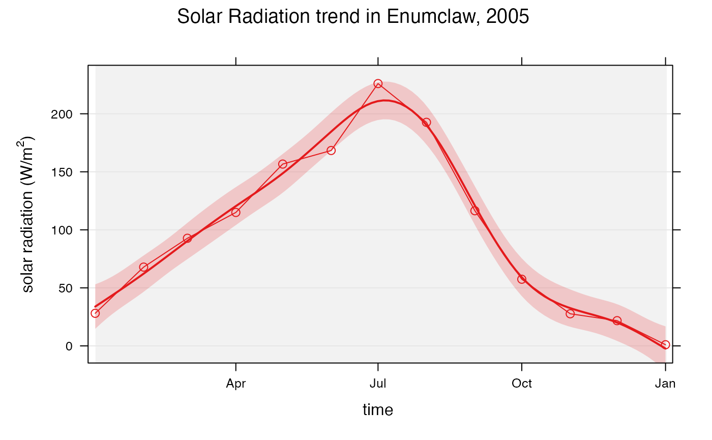
Plotting trends in data is also very easy using
openair. The smoothTrend() function plots
monthly averages against the trend in the variable of interest. Lets
look at the trend of solar radiation in Enumclaw in 2005:
openair::smoothTrend(
  enumclawData_2005,
  pollutant = "solarRadiation",
  avg.time = "month",
  main = "Solar Radiation trend in Enumclaw, 2005",
  statistic = "mean",
  xlab = "time",
  ylab = expression('solar radiation (W/m'^2*')')
)
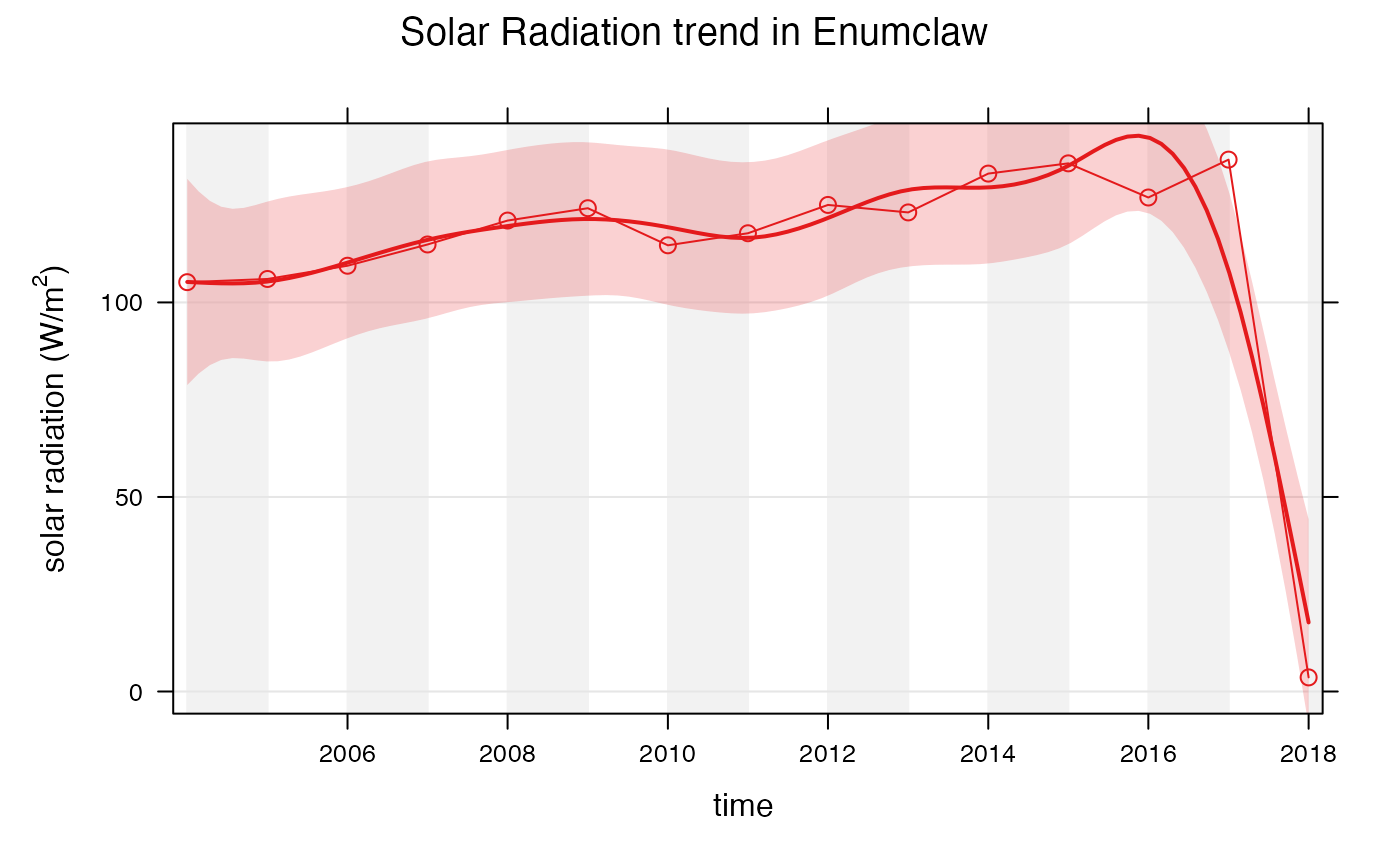
Instead of comparing monthly averages to the trend of the data, openair can also compare different averages.
openair::smoothTrend(
  enumclawData_ALL,
  pollutant = "solarRadiation",
  main = "Solar Radiation trend in Enumclaw",
  statistic = "mean",
  xlab = "time",
  ylab = expression('solar radiation (W/m'^2*')'),
  avg.time = "year"
)