PurpleAir Time Series Data
Mazama Science
2023-03-16
Source:vignettes/articles/pat_introduction.Rmd
pat_introduction.RmdTime series data provides a minute-by-minute database structure for transforming and analyzing PurpleAir sensor data. This vignette demonstrates an example analysis of an individual monitor located in Seattle, Washington over a two-month duration in which the Pacific Northwest experienced hazardous air-quality conditions caused by wildfires in British Columbia, Canada.
Disclaimer: It is highly recommended that you read
vignettes/pas_introduction.Rmd before beginning this
tutorial.
Loading PurpleAir Timeseries data
PurpleAir sensor readings are uploaded to the cloud every 120 seconds
where they are stored for download and display on the PurpleAir website.
After every interval, the synoptic data is refreshed and the outdated
synoptic data is then stored in a ThingSpeak database. In order to
access the ThingSpeak channel API we must first load the synoptic
database, but for the purposes of this example, we are going to use the
example_pas associated with the AirSensor
package.
library(MazamaCoreUtils)
library(AirSensor)

# Define PURPLE_AIR_API_READ_KEY in a .gitignore protected file
source("global_vars.R")

# Use an existing 'pas' object
pas <- AirSensor::example_pas

# Create a new 'pat' object
pat <-
  pat_createNew(
    api_key = PURPLE_AIR_API_READ_KEY,
    pas = pas,
    sensor_index = "3515",
    startdate = "2022-07-01",
    enddate = "2022-07-08",
    timezone = "UTC",
    verbose = TRUE
)
Notice that when passing our synoptic dataframe “pas” to
pat_createNew(), we also supply a senor_index
and a date-interval. In this case, our monitor-of-interest (MOI) has
sensor_index “3515” and our dates-of-interest are 2022-07-01 to
2022-07-08.
The PurpleAirTimeseries (“pat”) Data Model
Let’s begin by exploring the attributes of the dataframe returned by
the pat_createNew() function.
## [1] "meta" "data"pat contains two dataframes, meta
and data.
The meta dataframe contains metadata of the selected
PurpleAir sensor – this includes non-time series data such as location
information, labels, etc. The data dataframe contains
datestamped sensor readings of PM2.5, temperature, humidity, and other
pertinent sensor data.
We’ll start by plotting PurpleAir’s raw sensor data. We can quickly
display the time series data by using pat_multiPlot() and
passing in our raw pat and desired plot type
(“all” sensor data).
pat %>%
  pat_multiPlot(plottype = "all")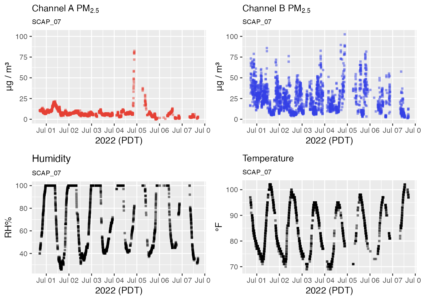
Exploring Time Series Data
Our pat dataframe spans two months. While this provides
a great overview of PM2.5, it is unwieldy to analyze if we are only
interested in anomalous air quality. We can use
pat_filterDate() to subset our pat dates. In
this case, we’ll reduce our time range to 2022-07-02 - 2022-07-05.
pat_august <-
  pat %>%
  pat_filterDate(startdate = 20220702, enddate = 20220705)

pat_august %>%
  pat_multiPlot(plottype = "pm25_over")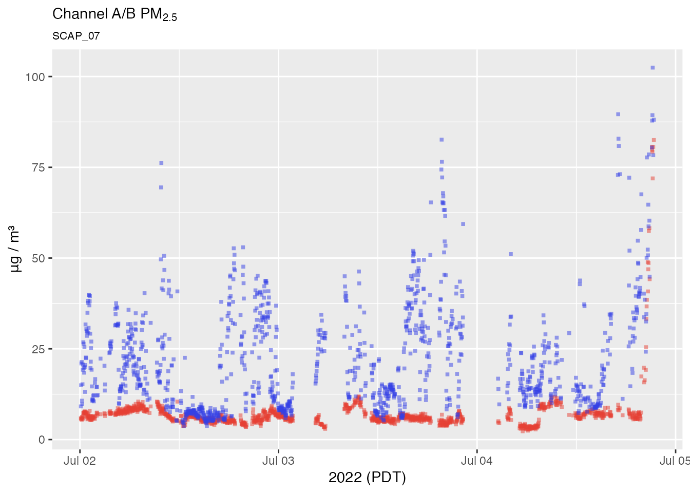
We can look for correlations in the raw data with
pat_scatterPlotMatrix(). When a sensor is properly
functioning, the only correlations will be a strong positive one between
between the A and B channels (pm25_A:pm25_B) and a strong
negative one between temperature and humidity.
  pat_august %>%
    pat_scatterPlotMatrix()
Outlier Detection
Our pat_august “pat” object displays some intermittent
sensor errors that appear as spikes in the data. In order to identify
and remove PM2.5 outliers like these we can use
pat_outliers(). By default, this function will create a
plot of the raw data with outliers marked with a red asterisk. It can
also be used to replace outliers with window median values.
pat_august_filtered <-
  pat_august %>%
  pat_outliers(replace = TRUE, showPlot = TRUE)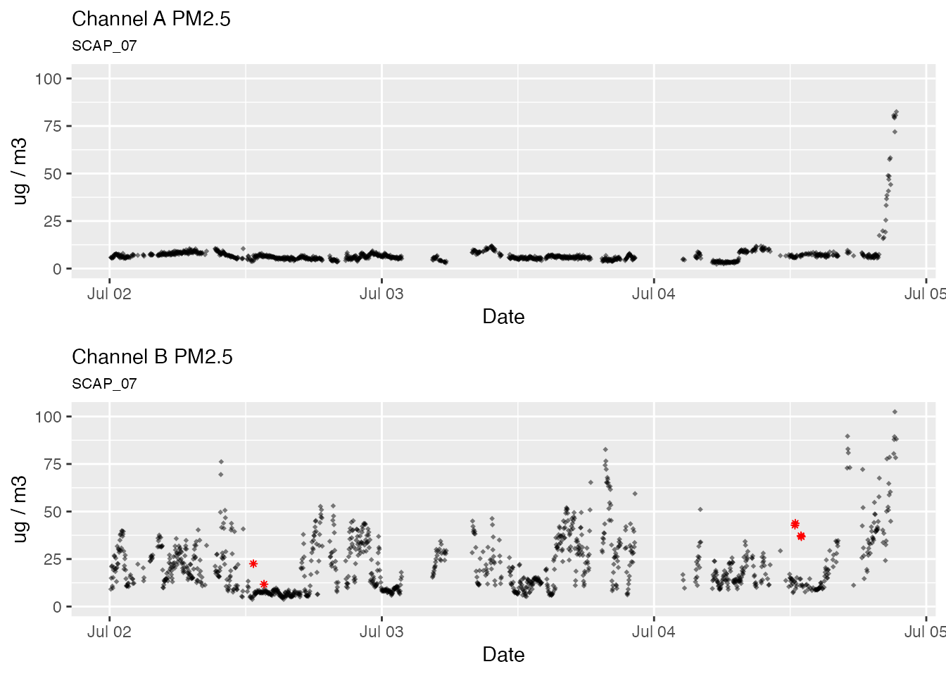
A/B Channel Comparison
Now that we have a filtered dataset we can subset the data further
and examine it in more detail. The pat_internalFit()
function will compare PM2.5 data from the A and B channels to verify
that the sensor is functioning properly.
three_days <-
  pat_august %>%
  pat_filterDate(startdate = 20220704, days = 3)

# Channel A/B comparison
three_days %>%
  pat_internalFit()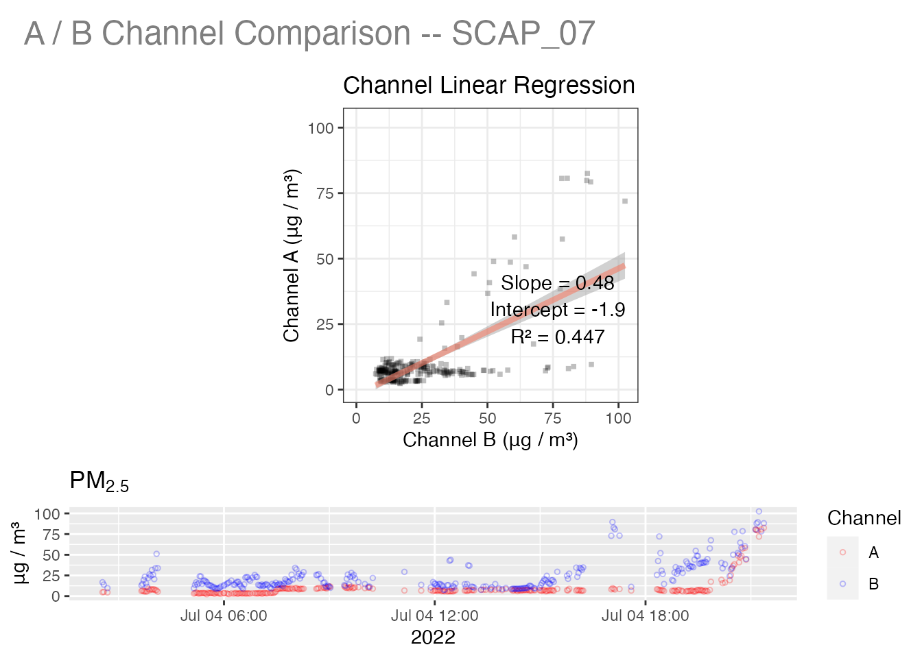
The high R2 value indicates that the two channels are highly correlated while a slope of ~0.9 suggests a slight relative bias in the measurements. (Perfect alignment would have a slope of 1.0.)
Comparison with Federal Monitors
For locations near federal monitors that are part of the USFS Monitoring site, we can also compare the sensor data with hourly data from a federal monitor
# Sensor/Monitor comparison
three_days %>%
  pat_externalFit()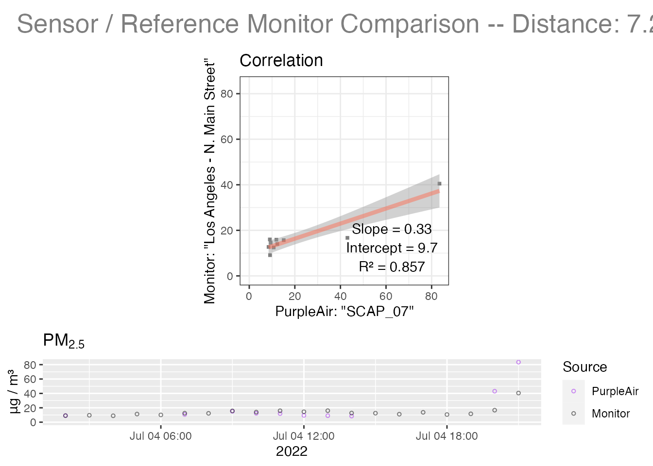
Overall, this is an excellent fit with the PurpleAir sensor capturing the temporal evolution of the wildfire smoke event impacting Seattle. The sensor data is biased a little high relative to the monitoring data but the much higher temporal resolution of the sensor provides a rich dataset to work with.
This package contains many additional functions for working with PurpleAir data and users are encouraged to review the reference documentation.
Happy Exploring!
Mazama Science