Creating County Maps

Mazama Science

February 4, 2020

Objective

The goal of this document is to introduce the countyMap() function in the MazamaSpatialPlots package. It demonstrates default usage and customizations using the countyMap() function’s arguments.

Default Plots

The countyMap() function requires three types of data. The first two are SpatialPolygonsDataFrames (SPDF) containing state and county level polygons. The SPDF containing state level polygons must include the variable stateCode in its @data slot. Similarly, the SPDF containing county level polygons must include the variable countyFIPS in its @data slot. The default state and county level SPDF’s are USCensusStates_02 and USCensusCounties_02 respectively, and are part of the package data. Higher or lower resolution US Census state and county SPDFs can be installed with:

library(MazamaSpatialUtils)
setSpatialDataDir('~/Data/Spatial')    # default directory for spatial data
installSpatialData('USCensusStates')   # state level polygons
installSpatialData('USCensusCounties') # county level polygons

The third dataset is a regular dataframe that contains the variable countyFIPS as well as a variable of interest. The variable of interest from this dataset is indicated using the parameter argument. This parameter is used to determine the colors of counties in the generated chloropleth map.

The next two examples demonstrate obtaining, summarizing, and mapping county-level data. The first uses an example dataframe from the package and the second demonstrates using read.csv() to pull data from the web and filling in missing countyFIPS using MazamaSpatialUtils::US_countyCodes.

Using package dataframe example_US_countyCovid

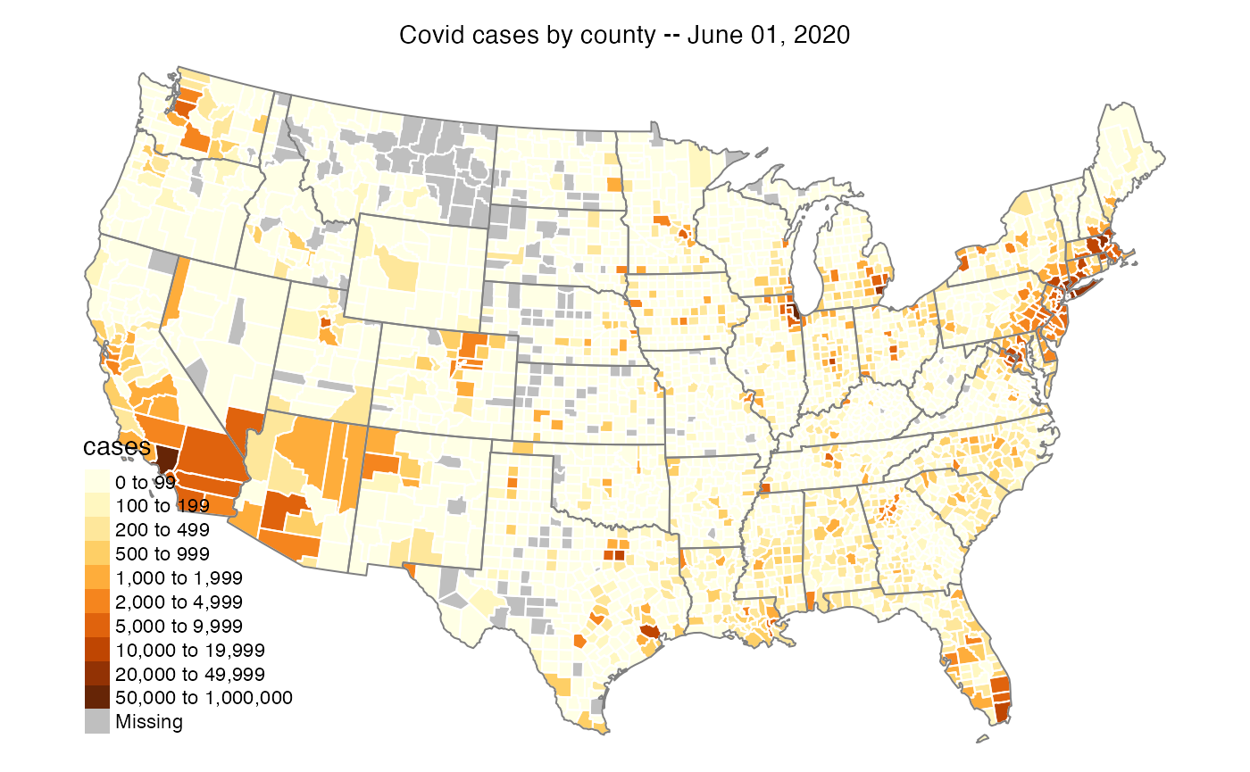
In this example, the package-internal dataframe, example_US_countyCovid, is used directly:

library(MazamaSpatialPlots)

countyMap(
  data = example_US_countyCovid,
  parameter = 'cases',
  breaks = c(0,100,200,500,1000,2000,5000,10000,20000,50000,1e6),
  state_SPDF = "USCensusStates_02", # the default value
  county_SPDF = "USCensusCounties_02", # the default value
  title = "Covid cases by county -- June 01, 2020"
)

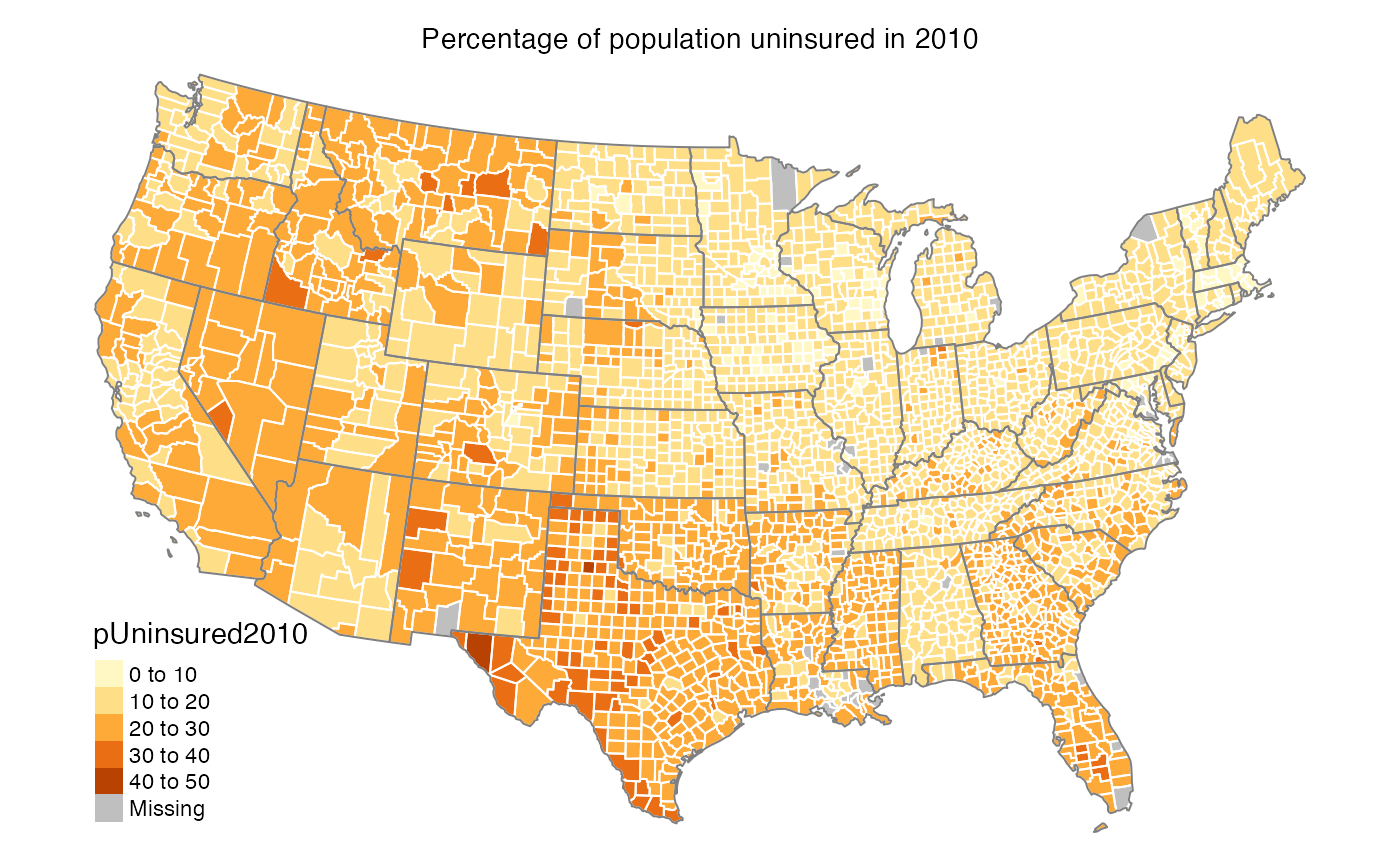
Using data found online

County level data of interest can be found online and easily loaded using read.csv() or scraped using MazamaCoreUtils::html_getTable() to parse all table elements from a website. Using these loading/scraping functions in conjunction with countyMap() makes it very easy to extract and visualize data from the internet.

# readme for data: https://healthinequality.org/dl/health_ineq_online_table_12_readme.pdf
URL <- "https://healthinequality.org/dl/health_ineq_online_table_12.csv"
characteristicsData <- read.csv(URL)

# Added required 'stateCode' and 'countyFIPS' variables
characteristicsData <- 
  characteristicsData %>%
  dplyr::mutate(
    stateCode = stateabbrv,
    countyFIPS = MazamaSpatialUtils::US_countyNameToFIPS(stateCode, county_name),
    pUninsured2010 = puninsured2010,
    .keep = "none"
  ) 

# Create map
countyMap(
  data = characteristicsData,
  parameter = 'pUninsured2010',
  title = "Percentage of population uninsured in 2010"
)

Customizing with Function Parameters

In the above examples, the countyMap() inputs data, parameter, state_SPDF, county_SPDF and title are used to create maps. This section will demonstrate how to use the other input parameters to customize your map.

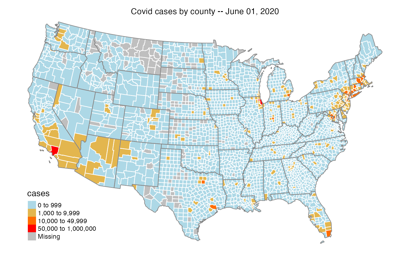
Using palette, breaks, and stateBorderColor

The palette, breaks, and stateBorderColor parameters dictate the coloring of your map. Colors are defined with palette and the distribution of color across the map is defined with breaks. As expected, stateBorderColor defines the state border color.

To make the most of these parameters, see the following references for R colors and palettes:

• http://sape.inf.usi.ch/quick-reference/ggplot2/colour

• https://www.r-graph-gallery.com/38-rcolorbrewers-palettes.html

In this example, breaks is used to create a coarser coloring scheme and palette is used to customize the exact color for each obesity rate level. The vector of breaks will be one longer than the vector of colors.

countyMap(
  data = example_US_countyCovid,
  parameter = 'cases',
  palette = c("lightblue", "orange", "red"),
  breaks = c(0,1000,10000,50000,1e6),
  countyBorderColor = "white",
  title = "Covid cases by county -- June 01, 2020"
)

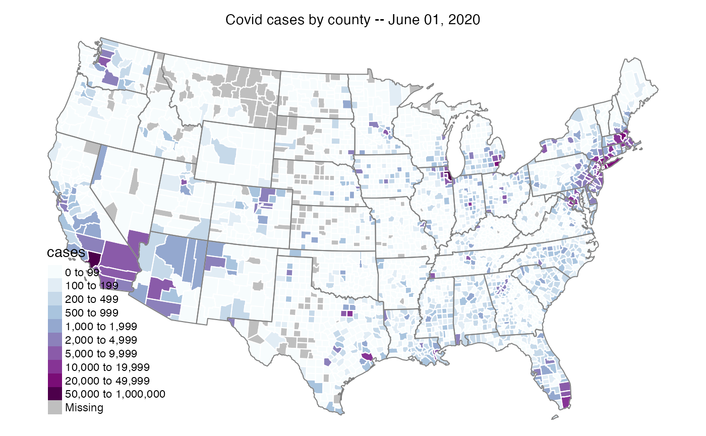
In this example, breaks is used to create a more detailed coloring scheme and the RColorBrewer blue to purple color palette name is chosen.

countyMap(
  data = example_US_countyCovid,
  parameter = 'cases',
  palette = 'BuPu',
  breaks = c(0,100,200,500,1000,2000,5000,10000,20000,50000,1e6),
  countyBorderColor = "white",
  title = "Covid cases by county -- June 01, 2020"
)

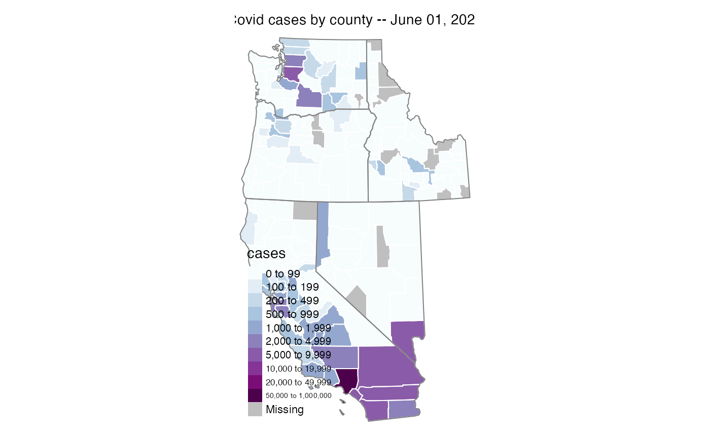
Using conusOnly and stateCode

The conusOnly and stateCode parameters define which states will be included in the map. If stateCode is defined, then conusOnly will be ignored. If stateCode is not defined, then conusOnly specifies whether the map is limited to the continental US. When conusOnly = FALSE, the continental U.S., Alaska, Hawaii, and U.S. Territories will be included.

This example builds upon the previous example and includes stateCode specification to create a map of Western states.

countyMap(
  data = example_US_countyCovid,
  parameter = 'cases',
  palette = 'BuPu',
  breaks = c(0,100,200,500,1000,2000,5000,10000,20000,50000,1e6),
  countyBorderColor = "white",
  stateCode = c("CA", "NV", "OR", "WA", "ID"),
  title = "Covid cases by county -- June 01, 2020"
)

Conclusion

The countyMap() function allows us to create attractive maps with a minimum of effort. When used alongside loading and scraping functions such as read.csv and MazamaCoreUtils::html_getTable(), U.S. county data can be procured and visualized in very few lines of code. Similarly to stateMap(), county level choropleth maps can be customized by harnessing the functionality of the tmap package.